Probabilistic Programming

” Probabilistic programming is one of most promising areas at the frontier of AI since the advent of deep learning. “ - Zoubin Ghahramani, chief scientist and vice president of AI at Uber and a professor at Cambridge University. (Published at MIT News)

In this neoliberal economy, the market capitalism is often expressed in terms of how much data a company holds. There is recorded information about anything and almost everything that steers current market and at times creates a new market. Content consumption has thus become most important driving factor. Fine ability to accurately model data and draw inferences has developed industry giants.

This modelling is studied as being of a deterministic nature or Probabilistic nature. Most of Machine learning advancements till now follow a deterministic approach to create inferences. However, the probabilistic systems follow a probability based approch, where there is added uncertainity about occurence of a particular event. Probabilistic algorithms are still being developed to craft the real world uncertainity.

The recommendation systems is one of the basic application of machine learning develpment and are continuously developed and studied. The authors of The Netflix Effect explain that recommendation systems tend to “steer the user towards this content, thus ghettoizing the user in a prescribed category of demographically classified content.” Precisely the recommendation system following a deterministic approach do not care about the undeterminism and uncertainity of a user’s mood and it tries to present him/her a recommendation that is based on several other users of alike tasefulness. It needs to be clearly understood that deterministic methods follow a total maximum number of liked/disliked content to present a suggestion whereas a probabilistic methods would recommend on the basis of probability. This would thus create an immediate shift in the recommendations. This is beautifully explained in this video talk by Prof. Christopher Bishop, where he explains that “getting causality from data is really a subtle and a really hard problem”. Such stochastic methods become more and more prevalent, thus determinism may be harmful. Probabilty based machine learning development may therefore help in advancing this.

In this blog we will try to understand the probabilsitc programs by a programming language theory approach, building upon basic semantics and then discussing some high level operational behaviour.

Please note that, we will not discuss any probabilisctic machine learning algorithm and restrict ourselves to semantic understanding of probabilistic programming languages.

Current Works :

Example Uses :

Recursive Multi-Agent Reasoning
Constrained Simulation
Breaking Captchas : A non-probabilistic programming approach would require gathering a very large number of Captchas, hand-labeling them all, then designing and training a neural network to regress from the image to a text string (Bursztein et al., 2014). The probabilistic programming approach in contrast merely requires one to write a program that generates Captchas that are stylistically similar to the Captcha family one would like to break – a model of Captchas – in a probabilistic programming language.

Let’s now discuss on the development of such probabilistic programs.

Starting off with a simple comparison of probabilistic programs with simple computer programs, We have :

Classical Computer Programs	Probabilistic Programs
Parameters	Parameters (probably in form of probability Distributions)
Parameter Analysis and Algorithm Implementation	Observe and Query
Checking Conditions	Check the Conditions (bottleneck & impossible conditions)
Program Output	Inferences

and a simple Syntactical Comparison would be something like :

Simple Imperative Programs	Probabilistic Progams

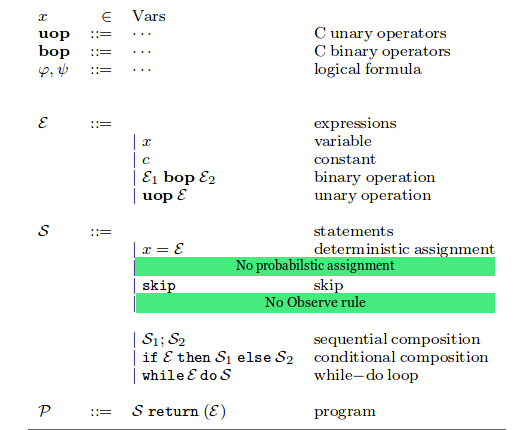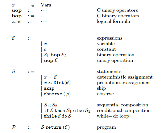We know that the likeliness of happening of an event is attributed to its Probability Distribution Function (PDF). We can asses a certain kind of outcome by querying and Observing the Probability Distribution. Taking the example of coin toss with a model based reasoning approach, there are two outcomes of a coin toss, a Head or Tail. Now let’s assume that the outcome is biased and the biasing function is a constructed off by a given number of variables. This forms a Bernouli Distribution. Then outcome may be understood as :


+-------------+      +-------------------------+        +---------------------+ 
|             |      |                         |        |                     |
| variables --+------+-> Biasing function      |---->   |   Outcome           |  
+-------------+      +-------------------------+        +---------------------+

Mathematically,

\( X = PDF(\alpha , \beta , \gamma) \)

\( Y = Binomial(X) \)

Here, X computes a bias in form of probability distribution. Y then inputs this probability distribution to Binomial’s distribution( to mimic the 0 or 1 case of coin flip) to result in a probability having a likelihood of 1 or 0.

We may then query a particular outcome as : \( P(X>0.6 & Y=1)\) , read as probability of getting a heads with having bias > 0.6.

A similar code in a simple imperative language as :

In a real world case this simplicity is hard to attain. It is important to note that these are first order programs. Higher order recursion is hard to achieve even with current languages.

Bayesian Networks and Discrete Time Markov Chains are often studied in probabilistic programming because of similarities, with the former being easily understood in terms of loop-free probabilistic programs and latter as a loopy probabilistic program.

Bayesian Network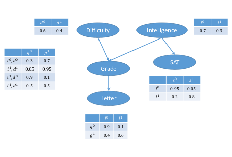
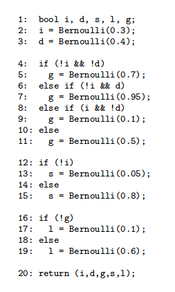Discrete Time Markov Chains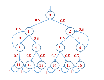

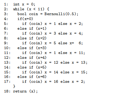(quoted from Probabilistic programming - MSR)

There are two kinds of inferences strictly based on generation (synonym to program outputs for non-probabilistic programs) for probabilistic systems :

Static Inference : This approach tends to compile probabilistic programs to probabilistic models like Bayesian Networks and then perform observation via inference algorithms.
Dynamic Inference : This approach tends to sample probabilistic programs many times over valid running conditions and observe an approximation to desired distribution.

Now that we have an idea of syntax representation and runtime outputs, let’s discuss about the working semantics of such probabilistc programs. It involves propagating data as probability distributions and symbolically executing statements and merging data flows following a required intention. Broadly, it may be studied as:

Static Analysis :

Similar to the case of static analysis of simple non-probabilistic programs, We create a decision diagrams to analyze the data flows. First order probabilistic programs specify probabilistic models over finitely many random variables. In this part we focus on the translation of these programs into finite Decision Diagrams or graphical models. Then we can see how this translation can be exploited to adapt inference algorithms.

Using a tuple notation for models, translation can be represented using a ternary relation \( \downarrow \) as :

\[ \rho,\phi,e \quad \downarrow \quad G,E \]

where,

\(\rho \) is a mapping from procedure names possibly used in the expression to their definitions.

\(\phi \) is a logical predicate for the flow control context, handling the parameters’ validity.

e is the expression we intend to compile.

This expression is translated to a graphical model G and an expression E in the deterministic sub-language which does not involve any sample or observe statements. E also represents the final value of the expression e in terms of random variabels in G. The vertices in G represent random variables and defines a probability distribution. It can be understood as weights in a graph.

Different Inference rules following classical \({ \frac{top}{bottom} } \) expressions, can be developed. Let’s discuss possible semantic rules for sample and observe commands.

Sample : It can be understood as a 3 step process,
- First, we translate e to a model with deterministic expression E . It should be clear that both e and E represent same probability distribution.
- Second, we choose a set of random variables of the network.
- Finally we convert the expression E into probability density or mass function F of distribution.
Observe : It can be understood as,
- Similar to sample, we create a density function F.
- Given a check condition, F may be reconstructed by slightly modifying G.

It should be noted that these are simply two kinds of command statements used to draw probabilistic inferences. In Static analysis method, we attempt to describe their working semantics, how will these 2 commands actually be expressed during execution. It should not be confused with the dynamic inferences as discussed earlier.

We would see in follwoing section the use of sample and observe commands to develop inferences during runtime.

Dynamic Analysis :

The main challenge of Dynamic analysis is to smartly reject out vague distributions so as to avoid unnecessary computation. These evaluation based methods performs improved sampling at every stage and propagating observations onto next probabilistic assignment. It consists of two steps :

Propagation of inferences through a pre-image operation analysis. It seeks to preserve the original program semantics. It can be realized by having an observe command to evaluate every inference.
Perform Sampling over transformed probabilistic programs. These can further be studied as :
- Likelihood weighting : This is the simplest method that involves tuning some of the variables of G to improve programs. It aims to approximate the posterior distributions with a set of weighted samples.
- Metropolis-Hashtings : This method uses the definition of aceptance ratio based on different factors. Struggle is improving the ratio.
- Sequential Monte Carlo : SMC sampling technique helps in case when there is a higher number of sample expressions.

Model Checking Probabilistic Programs

Probabilistic Model Checking involves checking through model checkers like PRISM if a probabilistic model satisfies a quantitative specification. Different Probabilistic models like Discrete Time Markov Chains (DTMC) , Continuous Time Markov Chains (CTMC) and Markov Decision Process (MDP) have been studied.